


We begin our journey into neural generative models with Diffusion models. In this exciting project, we leverage a pretrained model from DeepFloyd to generate images from inputs such as: text prompts, images, or pure RGB noise. Leveraging the pre-trained weights, we manually implement iterative diffusion denoising, Classifier-Free Guidance (CFG), and enhance the capabilities of the model via image-to-image translation, hole filling (inpainting), and explore how to achieve results similar to that of Visual Anagrams (Geng et al., 2024)
Utilizing DeepFloyd's Stage 1 function allows us to take the text prompts inputs and generate image outputs. Subsequently Stage 2 of the model we can implement super-resolution of our generated images. (YOUR_SEED = 400)
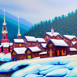
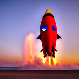
We notice that the model is able to generate images that are quite close to the text prompt.
However, these images were cherry-picked as the model is not perfect and can generate images that are not quite
what we expect. We also notice a propotional initial correlation between the quality of the image and
num_inference_steps.
First, we begin by creating our own forward pass that can add noise to an image. Given we are
using a pre-trained model from DeepFloyd, we need also need to adhere to two constraints: 1) The non-linear
noise schedule they used to train the model (using a look up table found within alphas_cumprod),
and 2) The number of discrete steps the model was trained with: 1000 steps (t values of 0-999)
More formally you aren't actually adding noise to the image, but rather blending between a noisy image and a predicted clean image. Unlike pervious projects were we blended the images like this: (A_img * selector) + ((1-selector) * B_img), in this case we square root the selector making the relationship not linear: (A_img * torch.sqrt(selector)) + ((1 - torch.sqrt(selector)) * B_img). The deviation of A and B are scaled down by the selector, but then added together. 'scaling' here is not referring to image size, but individual pixel values. Not yet quite sure why at the moment this non-linear relationship is better.
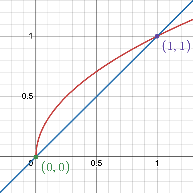
Of note is that the formula ∈ ~ N(0,1) does not mean that the noise generated is of range 0-1, but rather that the noise is of 1 standard deviation (generally values of -4 to 4). Here are the results from the forward function at the corresponding values:


Before overcomplicating things, one should always evaluate the simple solution: "Can we remove
the noise with convolved Gaussian filters instead of Machine Learning models?" The short answer is "not well
enough".
We manually tune the kernel size and sigma trying to strike the balance between getting rid of the noise while
not losing too much detail in the original image. Here are the results:


Now let's apply what we learned in project 2 by applying a sharpening filter to bring back detail by subtracting one gaussian level vs another and adding in the sharpness to the original image:
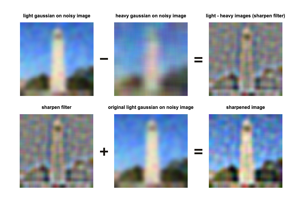
Unfortunately the infromation has been lost and cannot be recovered without some digital creativity. We will explore this in the next section.
To solve this problem we can utilize the unreasonable effectiveness of diffusion models and large scale datasets and compute to hallucinate the data lost by projecting the known pixels back into the manifold of images found in the dataset. In this section we do single shot prediction of what the noise is in the image and compute how to retrieve an estimation of the original clean image:


The only downside to the single shot denoisingthis approach is that as shown in the images above, The greater the noise in the image, the more the model struggles to predict the noise and causes blurrying in the output. We will tackle this in the next section where we iteratively reduce the noise in multiple diffusion steps.
Instead of the single shot
approach of predicting noise, we break this up into itertive denoising of the image. My intuition here is that
this architecture enduces the model to think in terms of coarse to fine detail.
In the section below, we compare the iterative diffusion, single shot diffusion and the simple blur approach. We
see that the diffusion approachs are generally much better than the blur approach and further that the iterative
diffusion approach restored additional details in the image; For example the definition in the foliage in the
background of the image. Given that the information is actually lost, the retoration process of the iterative
diffusion HAS to hallucinate the detail, leading to some creative interpretations of the original image.


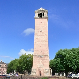
Instead of sampling from an existing image, we can hallucinate images from scratch by sampling from pure noise. My initial observation is that the the lower the stride → the richer the image is. Often a high stride (less iterative steps total) result in solid black or purple colored results. All images are enhanced used using super resolution.


We enhance the controlability of our generative model via the technique of Classifier-Free Guidance (CFG), which in a way
gives us a control knob to adjust the influence of the text prompt on the generated image.
Given that
our model has the capability to "see" which part of noise looks like a given text prompt, we can compute
the delta between a user given text prompt and an empty text prompt, scale that delta by the
cfg-scale, then add it to the unconditional noise.
The truly exciting concept ⭐ is that you can extrapolate outside of the manifold of images in the
original dataset
by choosing a CFG values higher than 1! Here you can see that CFG = 7 is literally giving you
other-worldy results: (I guess this alternate world is very purple) 😊


Now that we know how to project images and noise into the manifold of known images, let's explore the
manifold ⭐ a
bit more. A simple and philosophically intersting question we can ask is: What are some things that the model
thinks is visually similar to my input image?.
More technically, we project our input image into the manifold and explore the area around it via two variables:
1) Controlling the initial amount of noise in the input image via i_start and
2) The number of incremental diffusion steps (which allow it to walk further away from the original
noise).
The images below how the model hallucinates images that are visually similar to the input image. In practice we
see that the lower the i_start and stride, the furhter away we are to a visual
similary to the input image. What is non the less beautiful to see what visual associations the model has with
the input image.


Let's see more results with some additional input images. (The stride was kept at 30 for all images)


Another fantastic application we can explore is how to interpolate between two concepts such as
"realistic" to "cartoony". We achieve this by using the text prompt "a high quality photo" (which
implies a certain degree if realism) and then using a strong CFG value.


We see an incredible result! In the first row, between the i_start values of 4
and 10 we see
that the model arrived at a very similar generalization of the 'realism / cartoony' axis as seen in the book by
Scott McCloud, "Understanding
Comics".

Some additional inputs from hand drawn images. You can see that for the first result it struggles to project this imaginary creature into the manifold of known images. The second image is a bit more successful.


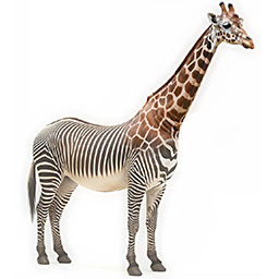
Using an input image as control, you can make some super rough visual edits to the image and hallucinate variations. In the first example we add a moon to the image and in the second example we add a river.
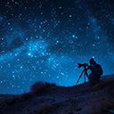
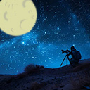
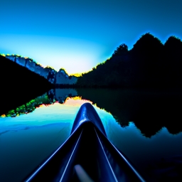
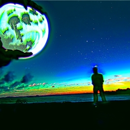
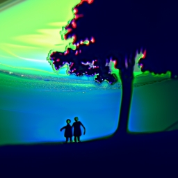
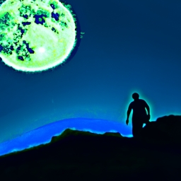
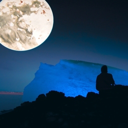

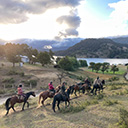
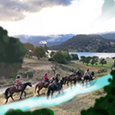
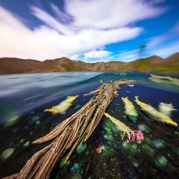
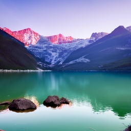
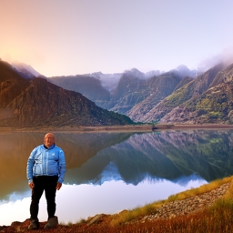
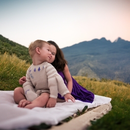
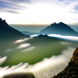
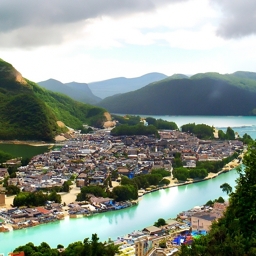
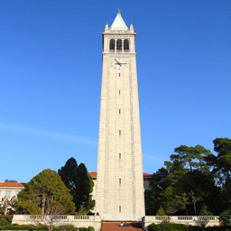
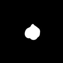
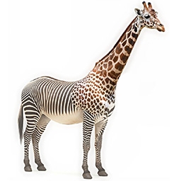
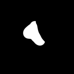
An emergent capability of this architecture is "hole filling" masks in images, known as inpainting. This is achieved by replacing the masked part of the pixels with the original image at each step of the diffusion. This forces the system to use the context of the original photo and inegrate it into the hallucinated parts.
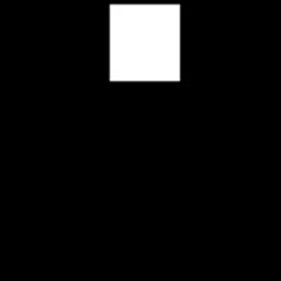
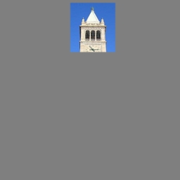

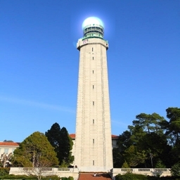
I was naturally curious how the inpaniting woudl work on the texture hybrid images from project 2. I think most of the images are an improvement! 😊

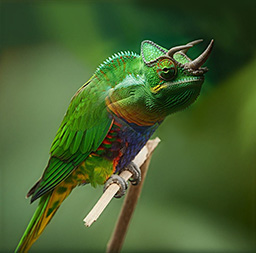


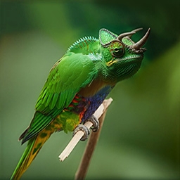
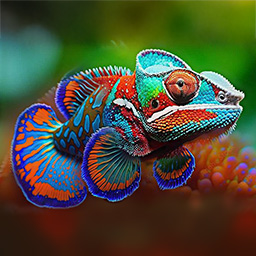

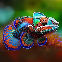
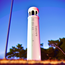
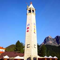
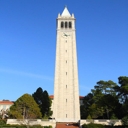
The other critical degree of controlability for this generative video language model is the 'languge' itself via the text promps. We can see that we can interploate between to locations in the manifold, one given by an input image and the other given by a text prompt. One easy way to understand what is happening in the images below is to think that when the amount of noise on the original image is high, it can get closer to the location of the text prompt, and the less noise the more it has to stick to what it already has (since it can't dramatically alter the image.)
Interpolation between the text prompt: "a pencil" and an image of a the Capmanile at UC Berkeley.
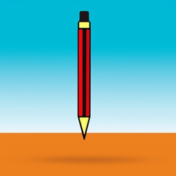
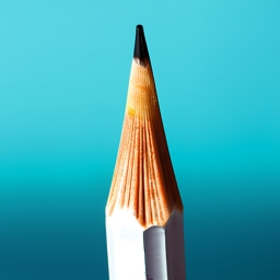

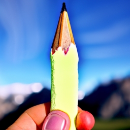
Interpolation between the text prompt: "a dog" and an image of rocks.
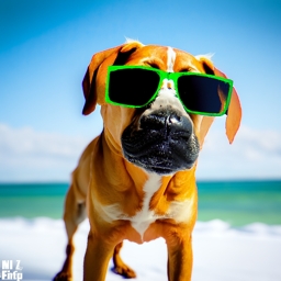
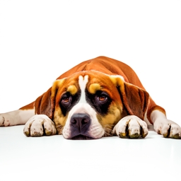
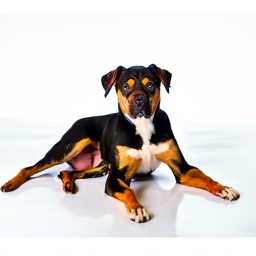
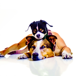
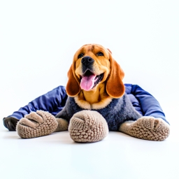
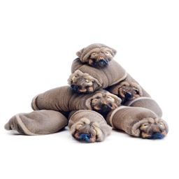
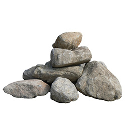
Interpolation between the text prompt: "a dog" and an image of cat.
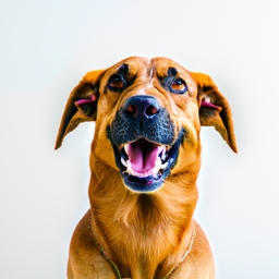
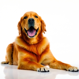
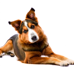
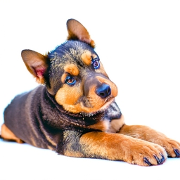
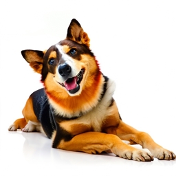

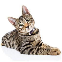
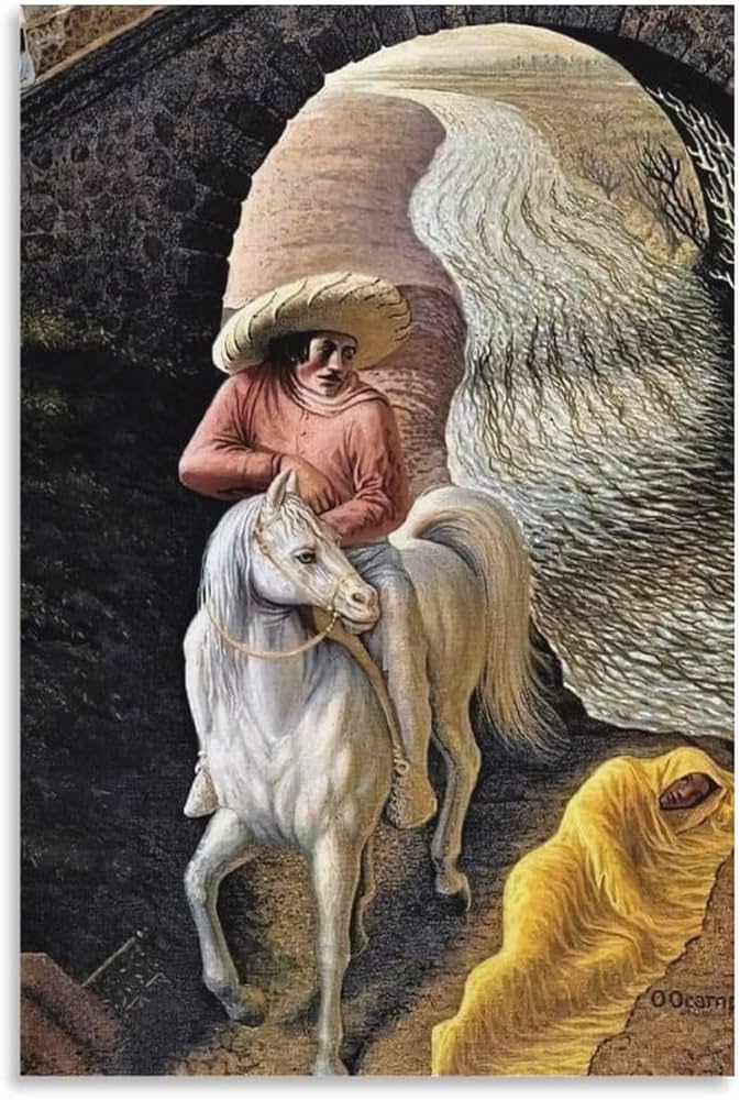
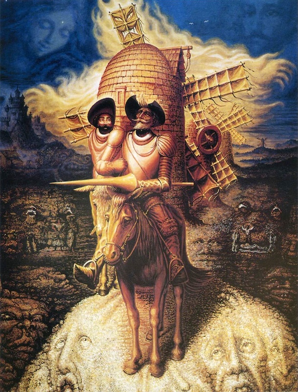
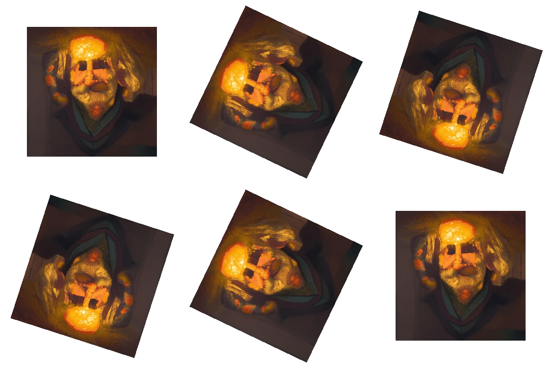
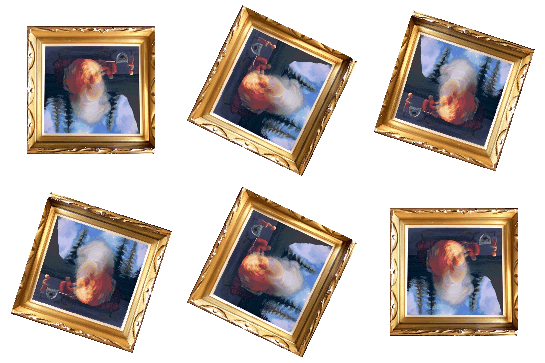
Similar to Mexican artist Octavio Ocampo's remarkable surrealist paintings from the 1970s, which reveal different images depending on the viewer's perspective, we will use our diffusion generative model to create dual-meaning illustrations. To achieve this, we will implement techniques from the Visual Anagrams paper (Geng et al., 2024).
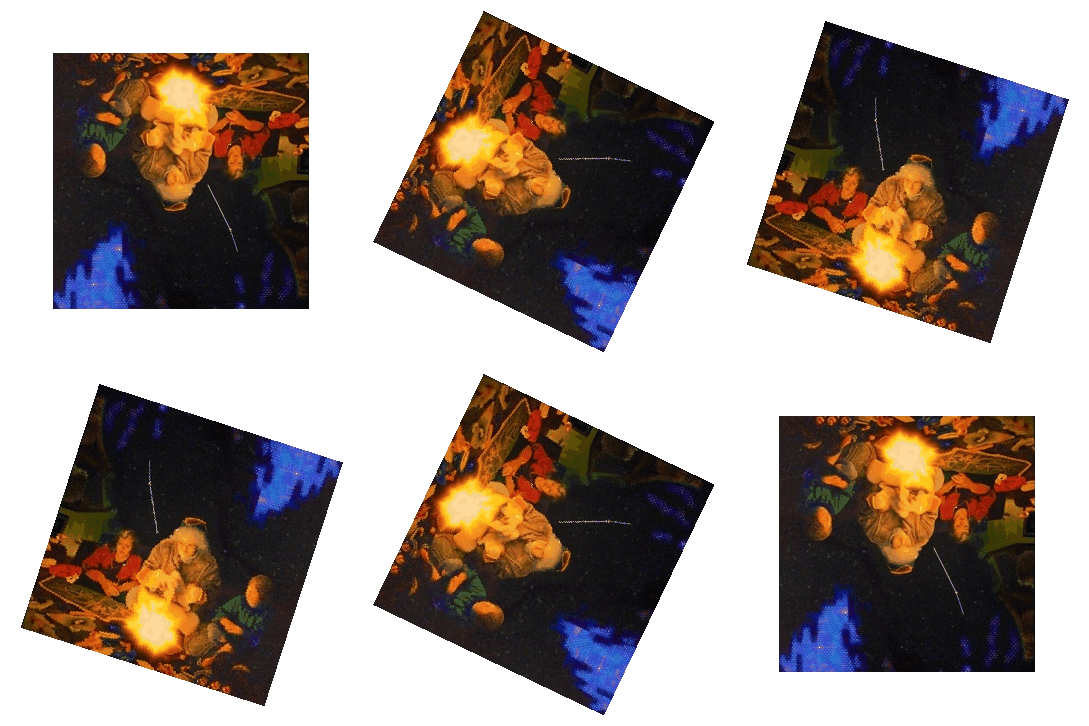
In order to achieve this illusion of dual meaning, during each iteration of the diffusion process, we follow the following steps:
This surprisingly simple technique yield some incredibly creative and striking!
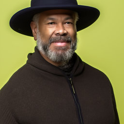
"an oil painting of an old man" → "an oil painting of people around a campfire"
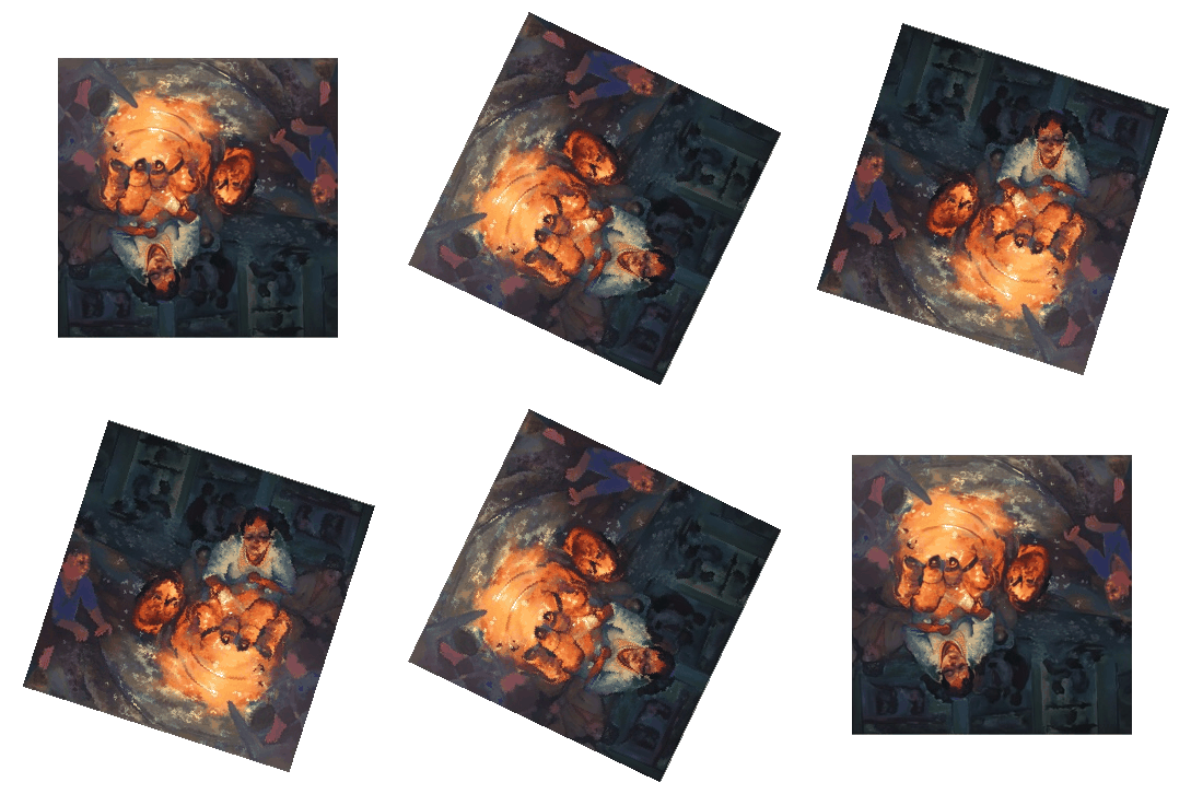
"an oil painting of an old man" → "an oil painting of a snowy mountain village"
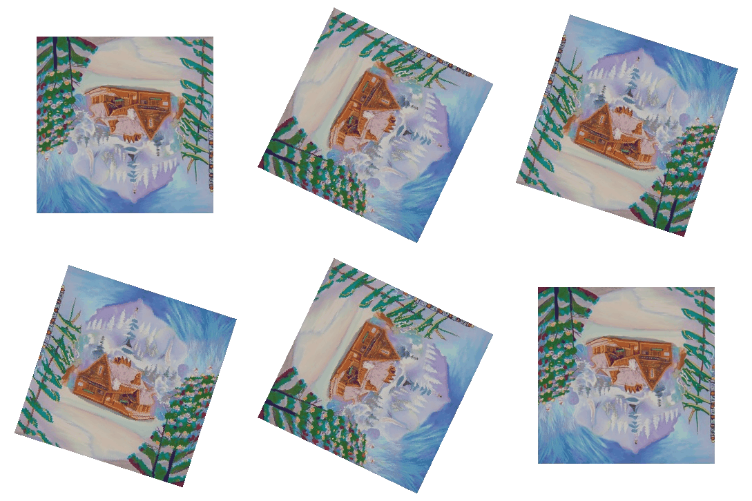
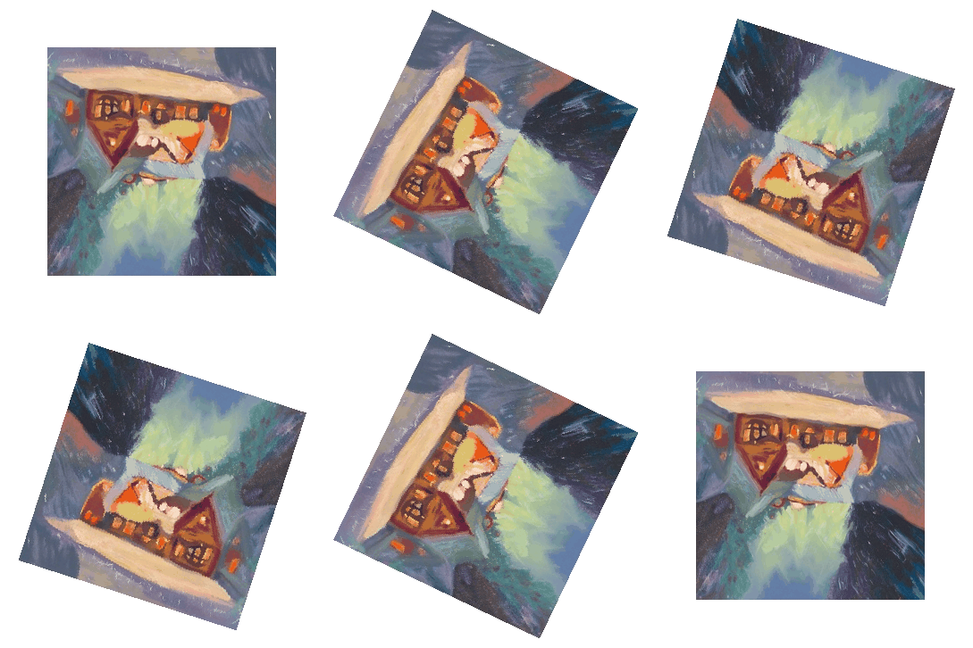
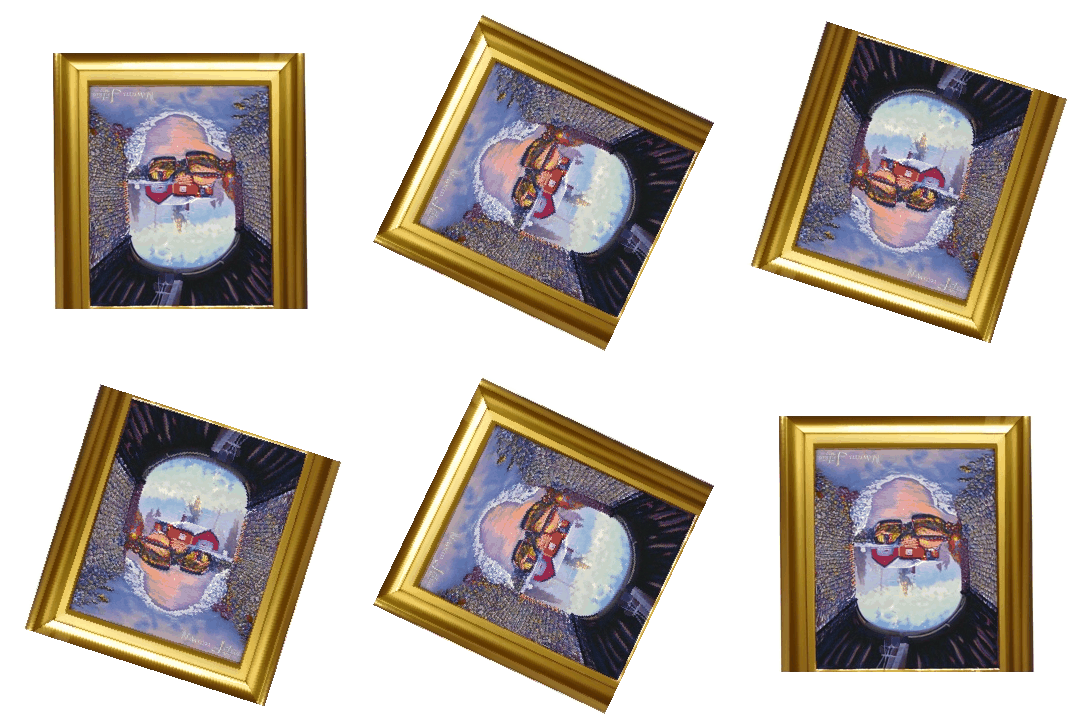
The first text prompt descriptions correspond with the large image, and second prompt corresponds with the small image.
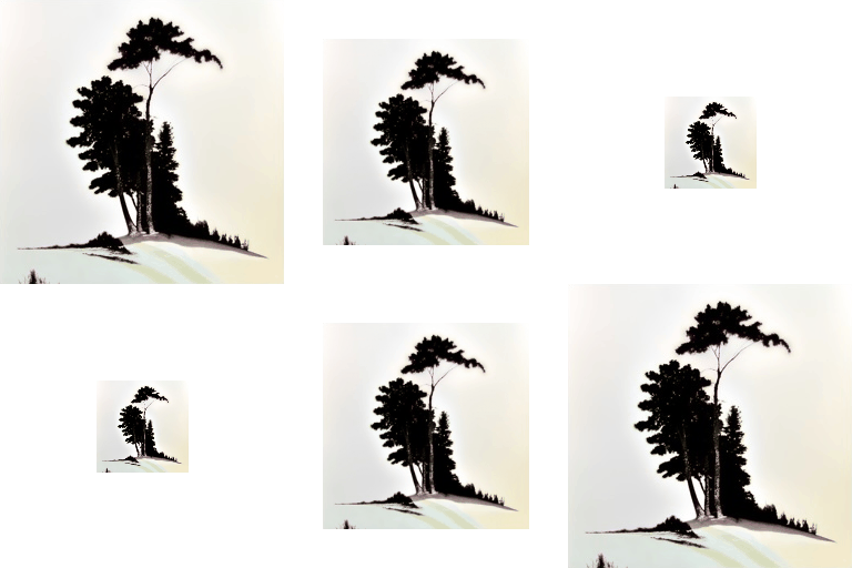
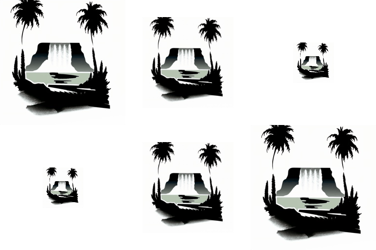
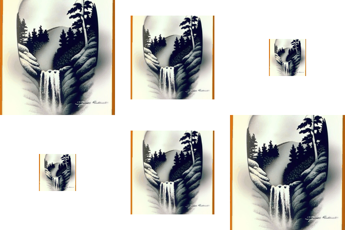
Now that we've gotten our feet wet playing with pre-trained models, let's try to implement a diffusion model from scratch! We'll start with a simple unconditioned unet model and then we will move to conditioning with time, class and re-implement Classifier-Free guidance.
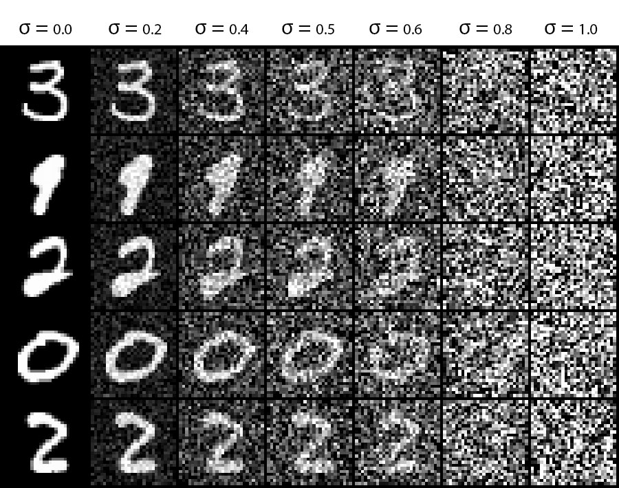
We being by 'diffusing' our original image with a noise function: Original + (normal noise * sigma):
We train a unet designed to predict the original image given a noisy image at simga = 0.5:
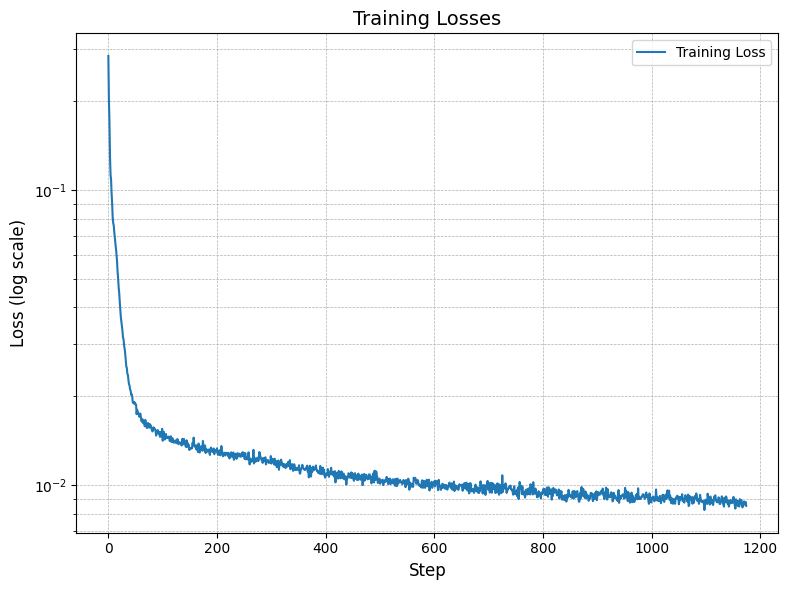
In the figures below you can see that the prediction capabilities improve with additional epochs:


However, given that this model was purely trained using simga = 0.5, it does not generalize well to other sigmas:

To boost performance across more sigma values, we train a time conditioned unet by noising the inputs to different t levels, and telling the model t level each image in the batch is at. So that this conditioning information is not accidentally lost in the encoding part of the architecture, we inject the conditioning data on the decoding (after the unflatten).
This time our models' goal isn't to directly predict the original image, but rather to predict the noise added to the image. Additionally like in Part A, we sample the model iteratively as to improve the details in the generations.
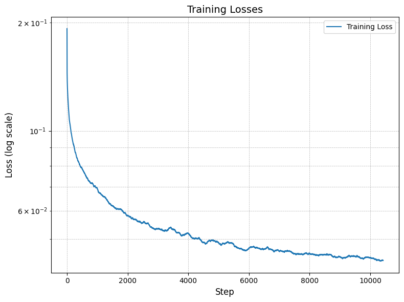
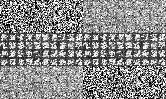
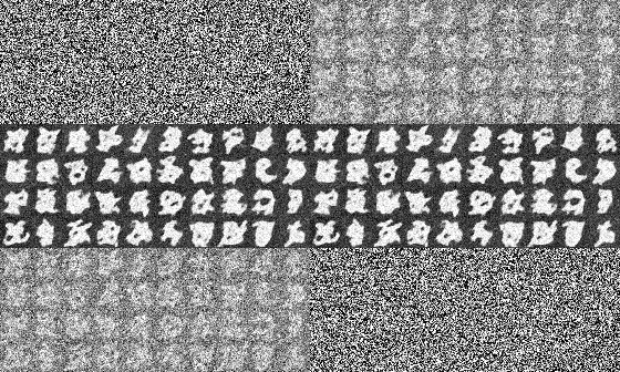
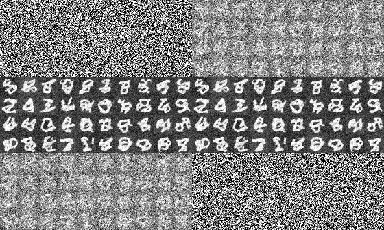
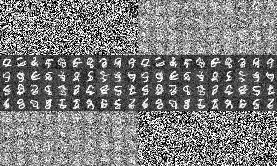
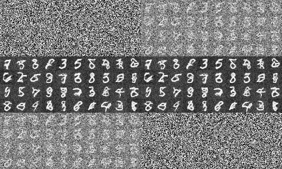
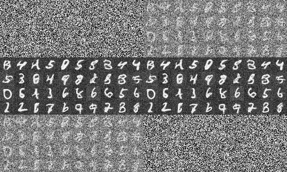
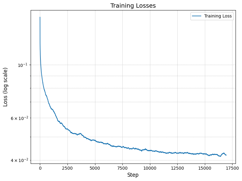
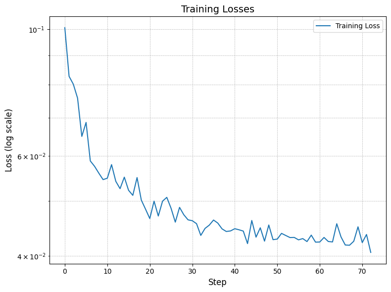
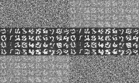
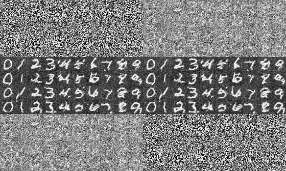
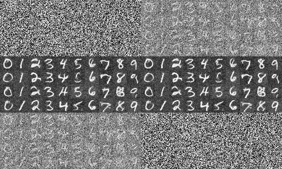
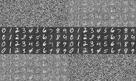
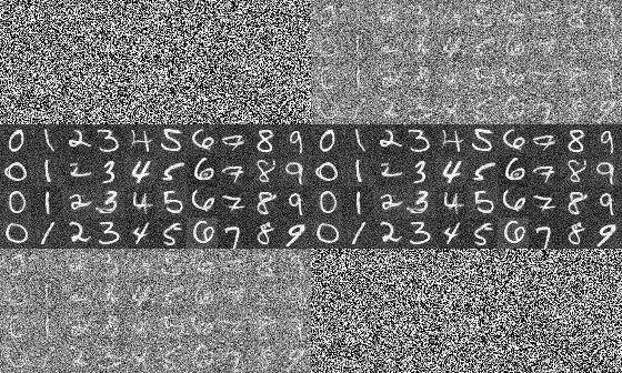
We continue to improve our model by adding class conditioning to the model. This is done by adding a one-hot enconding to the architecture at the same point where we injected the time conditioning. In order to incourage the model to work even without the class conditioning, we add a dropout layer to the class conditioning with a probability of 0.1. Here we also evaluate the test loss to make sure we are not overfitting.
While this was by far the most challenging project in the course, it was equivallently the most rewarding. With
other projects, you could predict what the output would be, but with this one, the results were always so fun to
look at. You truly begin to appreciate the power of neural networks and the potential of generative models. I
particularly enjoyed feeding the model noise and seeing it hallucinate images. This makes me think of "Do
Androids Dream of Electric Sheep?" by Philip K.
This was a fantastic forcing function to learn about pytorch, neural networks, and the diffusion models!