

When starting new projects, I like to ask myself two questions:
This led me to create a mock up by manually correcting perspective in Adobe Photoshop. From this I learned that:
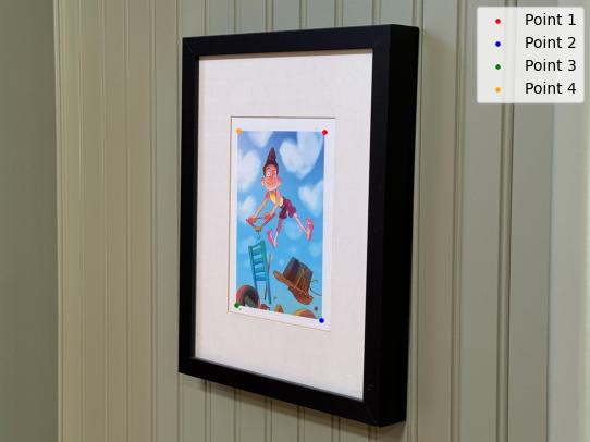
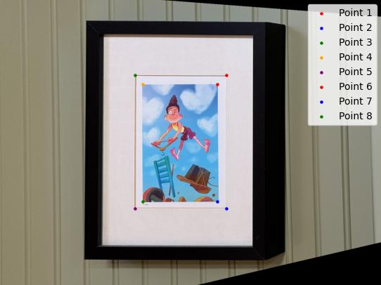
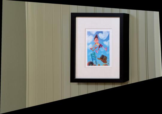
First I create correspondence between the original image and the desired image. Like the previous project, I chose to use Autodesk Maya to place my points of correspondence. This is useful as it allowed me to use sub-pixel accuracy. I then use the correspondence to compute the homography matrix. The "computeH" function figures out the homography matrix H, which shows how points from one image line up with points in another. Like previous student projects, I use Singular Value Decomposition (SVD) to solve for the transformation. The key info comes from the last row of V^T, which is reshaped into a 3x3 matrix. After normalizing it, you get the homography matrix that describes how to warp one image to match the other. Here are the results:
Since the target deformation wasn't square, I had to measure what were the ratios of the sides for the target.

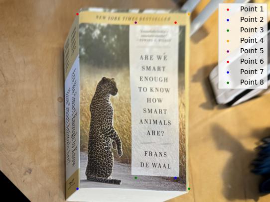

My favorite part of this project was starting to think about overspecified systems given and making guesses based on the power of larger amounts of data. For the challenges at first my pixel splatting was taking a long time and I couldn't figure out what was happening, and then I realized that my points of correspondence were not in the same order. I also had to manually create the points of correspondence which was a bit tedious. I can't wait for Project 4B to automate this and remove a lot of human error out of the equation.


ANMS picks important points in a picture by giving each one a “radius” that measures how far it is from stronger points nearby. Only points with the largest radii are kept, which means we end up with the strongest points that are also spread out, making it easier to line up or combine multiple pictures.


Luckily this technique is applicable outside the domain of photos of Kamala Harris.
Let's
use these technique for the utility of creating a stitched landscape mosaic of a room.
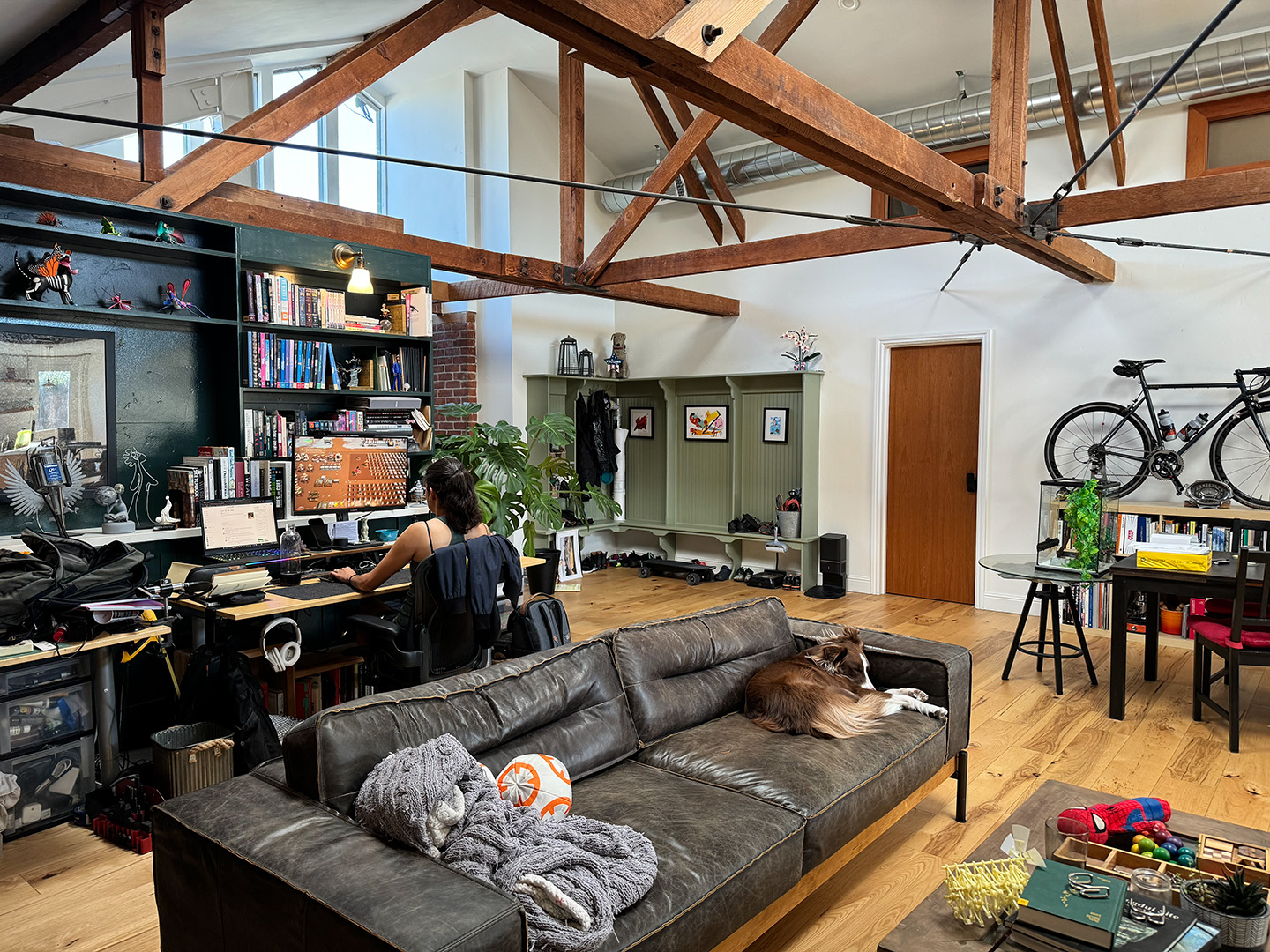
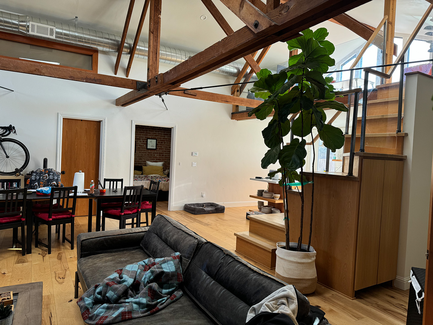
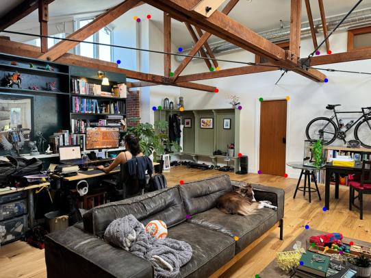
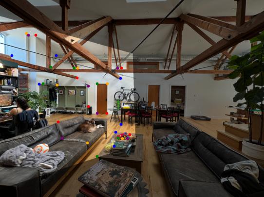
Here are the input images for the mosaic:


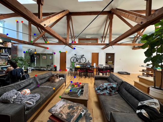
Previous alorithms applied to the room images result in the following correspondences:


And their corresponding Feature Descriptors:


Now that we isolated interesting differentiable patches in the image, we can start to
compare them to each other to find correspondences. To find the matches, per patch we calculate the L2
distance
(known as nearest neighbor in Machine Learning) between all pairs of descriptors and store them in a sorted
list. Instead of doing filtering based on global L2 distance between potential correspondences, we use the
method described in Distinctive
Image
Features from Scale-Invariant Keypoints. by David Lowe in which we use the ratio of the distances of
the
two best Nearest Neighbor matches. If the ratio is less than 0.8, we consider the match to be valid. This in
a
way gives "confidence score" in relation to the second best match.
Surprisingly this algorithm finds some corresponsances despite knowing the true alignment would
require perspective warp and that this algorithm is neither rotation nor scale invariant.

This could still use some improvement so let's use RANSAC to find the best matches. Here are the much improved results:

In reality, we use a much higher count of interest points to find a good homography. Here is first the feature descriptor matching:


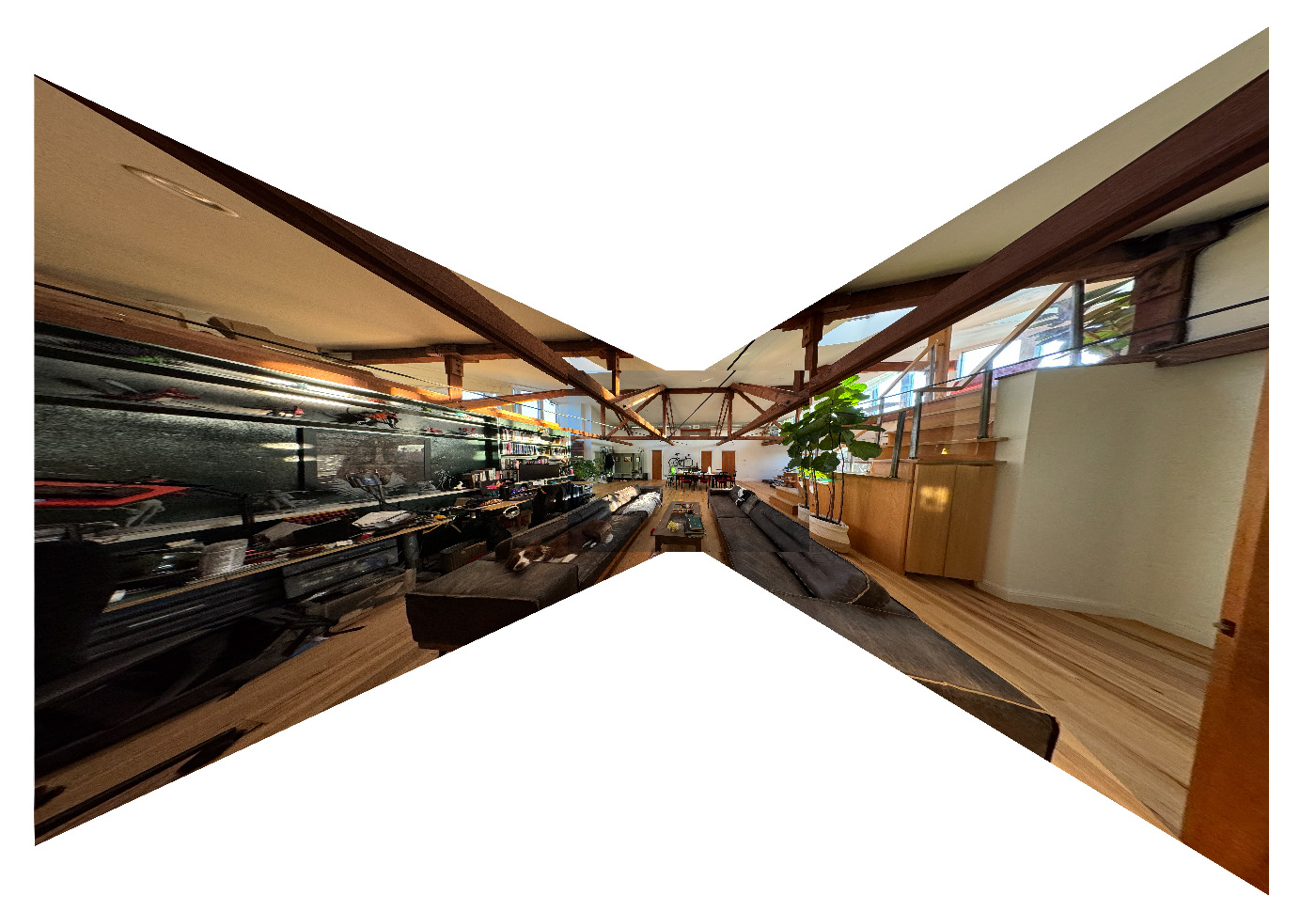
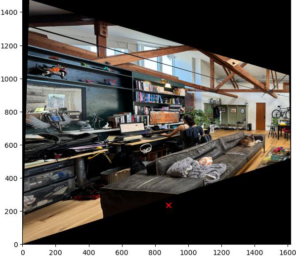
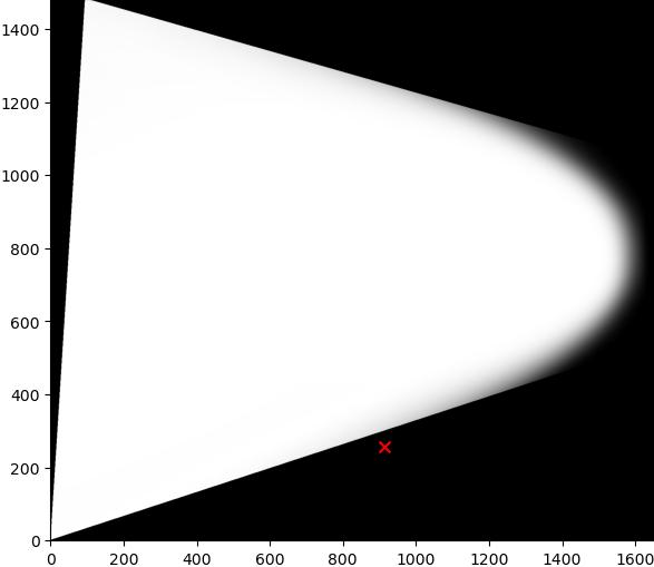
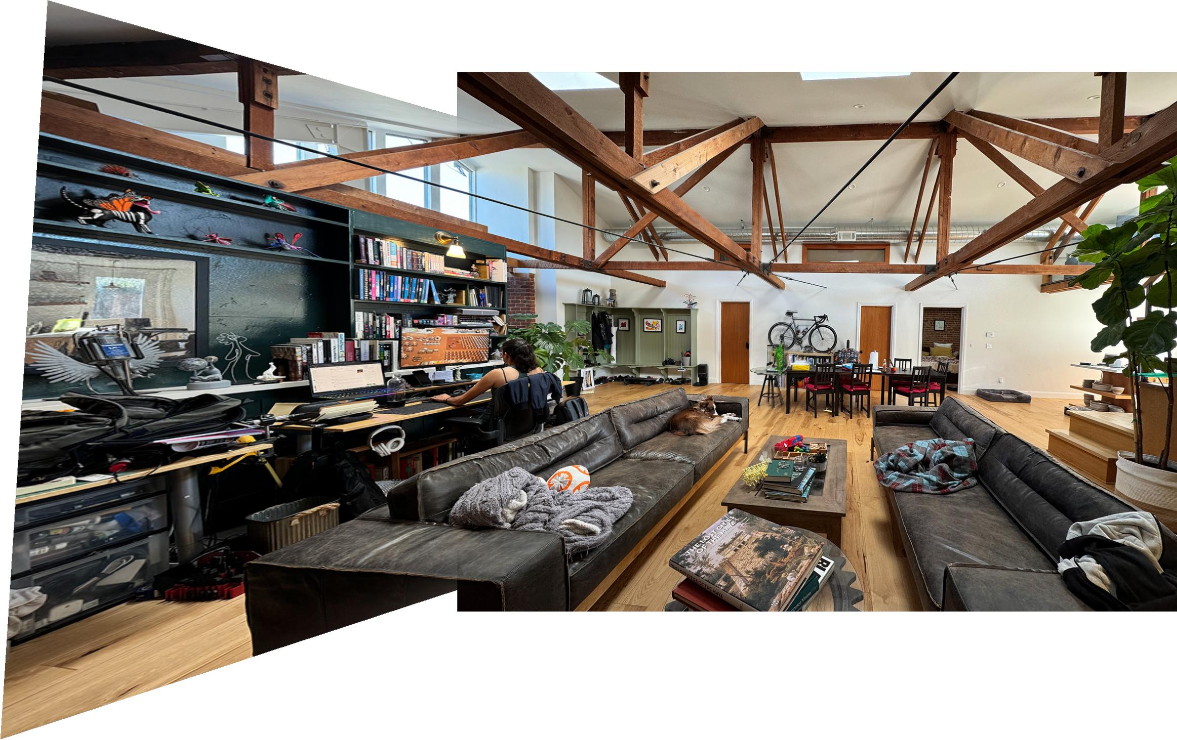
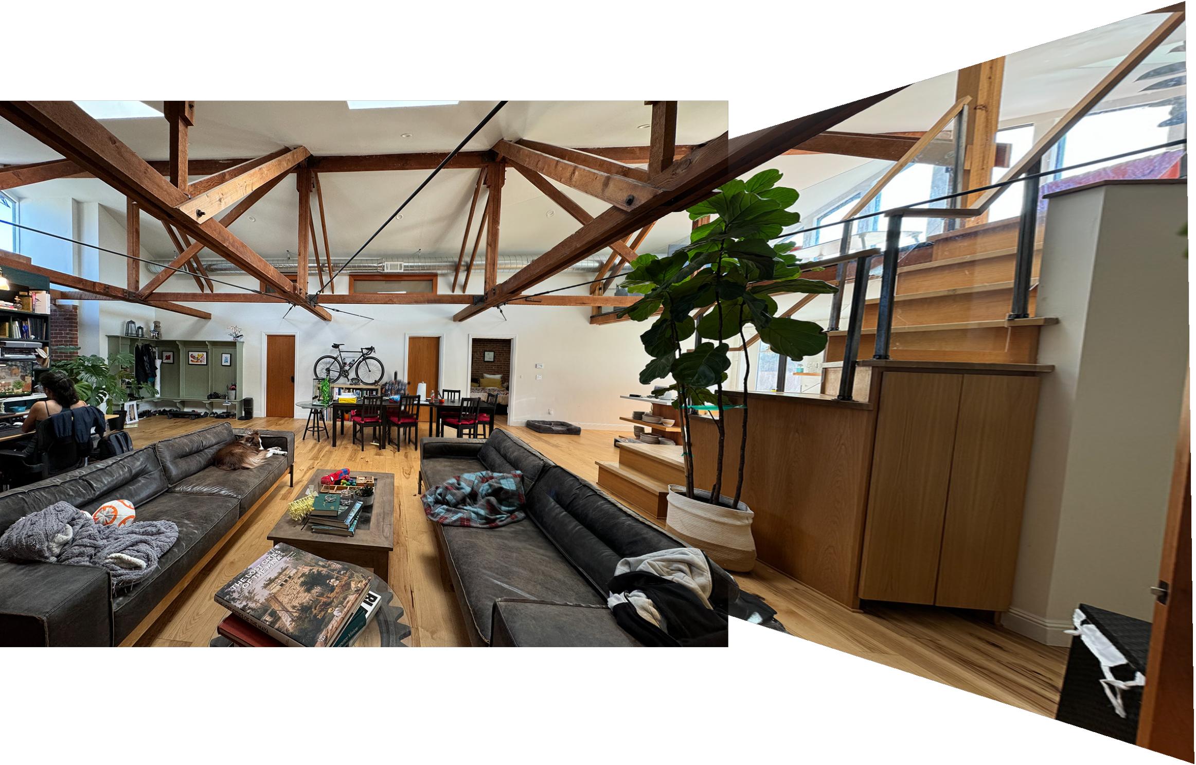
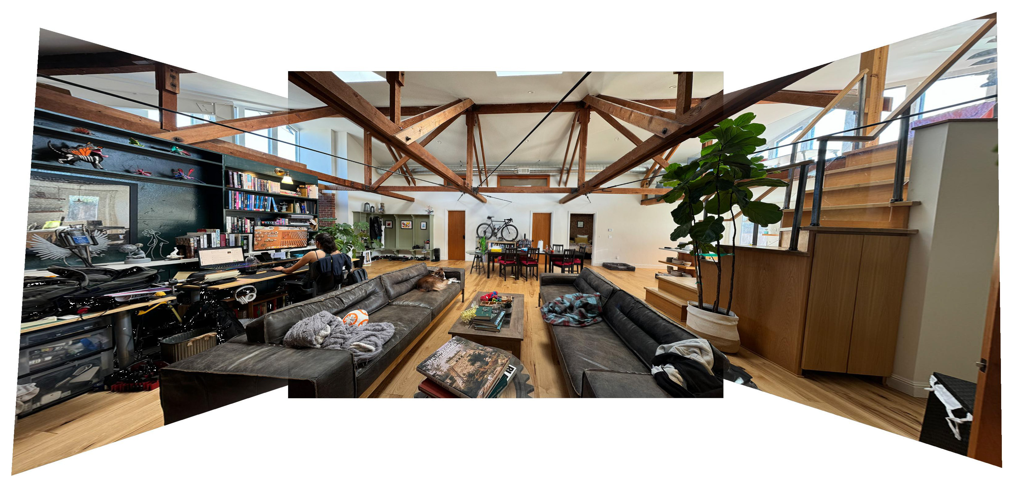
We then compute the homography warp per each pair of correspondences and stitch the images together. For the blending I used the same texture as in project4 which I think gives a nice result:


My favorite part was seeing how powerful RANSAC is even without rotation or scale invariance in the descriptors. Given we know for sure that to align the images it would require a perspective warp, it's impressive it works. My suspicion is that this is mostly because of the translation invariance from blurring the descriptors. Some challenges I had during this project were fighting with the non-standardization of X and Y order across libraries. Surprisingly figuring out how to expand the canvas and align the multiple stitches was harder than I thought it would be!